
Knowing the cost to acquire a single customer (Customer Acquisition Cost or CAC) is important for any business but especially e-commerce sites using Pay Per Click (PPC) advertising. If you run a Shopify store and use Google Ads or Facebook Ads, this tutorial will show you how to calculate an overall CAC and easily create a simple dashboard for sharing using Lido, the leading low-code platform based on spreadsheets that lets you build powerful internal applications and dashboards without needing developers.
In this tutorial we’ll show you how to:
Lets go!
If you don’t already have an account, first set up a free Lido account.
Opening the Starter File

Next, connect to your Shopify order data as a datasource in Lido:


We'll find ourselves back in the sheets view looking at our new live-connected Shopify data table! Our new Sheet is named “View~ShopifyOrders1~1”. Don’t change the name. (you can collapse the sidebar now by clicking on the “x”).
Our "live" connected Shopify orders spreadsheet table

Every time you open the file, the dataset will be refreshed with the latest data.
MAKETABLE
If you look in cell A1, you'll see one of Lido's powerful additions to Excel's standard formula's where all the magic happens - MAKETABLE.
Lets take a closer look. MAKETABLE creates a named table that can be manipulated, attached to dashboard components, filtered and more. Because MAKETABLE can be connected to a datasource such as Shopify and records will update in realtime, it's not possible to rely on static cell ranges (such as A1:C50) to make sure you have all of the data. With MAKETABLE, all you need to do is reference the name of the table.
What the function above says is "Make a table out of the Shopify datasource I have called "ShopifyOrders1" and we'll name this table "View~ShopifyOrders1~1", and just use the same column names as the datasource has already.
The function documentation is:

We'll run into MAKETABLE again later, but for now lets move on!
For the simple blended CAC we’re calculating, we’ll use the # of orders a day as our measurement. Blended means that we'll simply add our Google Ads and Facebook spend together and divide the sum by the number or Shopify orders for that day.
To do that, we need to group our Shopify by day and have a count of the # of orders.
Another one of Lido's powerful extensions to the standard set of Excel formulas is GROUPBY. Let's use the visual helper to use this formula.


Our Shopify orders are now grouped by day with a count of the orders.


The orders are sorted from most recent to oldest. We want to reverse that order so that our chart will look correct later on. Because of the GROUPBY function, we need to do a little extra work to sort it properly. We're working on an update to Lido to make this process more simple, but for now, do the following:
1. Strip the header columns off of the table.
We'll return to our MAKETABLE function and use another Lido function, SLICE, to remove the header row. Looking again at cell A1, the current MAKETABLE function looks like:
Now, wrap the GROUPBY function in a SLICE function to remove the top row.
What this SLICE function is saying is: "give me all rows, starting at the 2nd row, and include all columns". SLICE, like many functions starts its count at 0 instead of 1. This is called "0-indexed".
SLICE lets you select a portion of any table (or "array"). Here is the function reference:

You should now have just the grouped Shopify data without the headers (you'll have to reapply the date format ):

2. Next, wrap everything in a SORT function to sort the table by day ascending. SORT is a standard Excel / Sheets function.
The SORT formula says "Sort whatever I'm given by the 1st column in ascending order".
3. Finally, add back the columns at the MAKETABLE level. With MAKETABLE, the last parameter is an optional list of column names. You'll also have to select and format the date cells as in step 1 above.
Now, you have a sorted and grouped table of Shopify orders that is updated in realtime.

Next, we need to connect our Google Ads data to understand how much we spent to get those Shopify orders:
You should now see a new sheet created named “View~GoogleAds1~1” with your Google Ads data.

Your Google Ads data will refresh automatically each time the Lido file is opened.

To match up with our Shopify data we’ll need to also group our Google ad spend by day. We’ll do that using the same method as we did for Shopify data.

You should now have a table of your Google Ads spend per day:

We now need to connect your Facebook Ads account if you also spent money on Facebook ads to drive Shopify orders.

Each time you open your Lido file the latest Facebook Ads data will load.

We will create a spreadsheet table that combines the live-data we have from Google Ads, Facebook Ads, and Shopify to calculate the daily Customer Acquisition Cost (CAC).
We'll do this by adding additional columns to the Shopify Orders table we already have. Currently, It has two columns - Day and Order Count:

Lets add another column with the amount of Facebook Ad Spend per day.
Its easy to do this with another one of Lido’s powerful extensions to standard spreadsheet functions - COMPUTEDCOLUMN. COMPUTEDCOLUMN lets you automatically compute the value of a new column for every row in a table that grows as the table grows. We can use the helper button to get started.

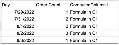
What this formula says is: "For every row in the table 'View-ShopifyOrders1~1', create a new column called "ComputedColumn1", and calculate the value by the spreadsheet formula - currently the placeholder text 'Formula in C1' ".
The function signature is:

RAW COMMAND can be any spreadsheet value or function. For now, replace the contents of the cell with:
For this, we’re just using good old XLOOKUP to lookup the current record's Day column in the View~GoogleAds1~1 table and return the total spend (the SUM column). You can think of XLOOKUP as the spreadsheet way to do a join in a relational database.
You'll see some new Lido syntax to reference table columns. Remember, MAKETABLE gives you a name for a specific table you can reference elsewhere in a sheet and that is what we're doing here.
View~ShopifyOrders1~1 is the name of the Shopify orders table that we created above with the MAKETABLE command.
@Day refers to the current row's value in the Day column.
View~GoogleAds1~1 is the name we've given to the Google Ads table
[Segments Date] is the way to refer to a whole column (without the '@') in another table.
So the way to read this XLOOKUP command is:
"Search in the Segments Date column of the View~GoogleAds1~1 table for the current row's Day value. If you find it, return the value of the SUM column. If you don't find it, set the value to 0"
When you’re done, you should have a table with a new column that brings in the Google Ads spend that looks something like this:

Remember, in Lido these tables are updated with live data, so if you have selected the last 30 days of sales, the tables will automatically update with the appropriate window of data.
To round out this table, add three more computed columns. Just copy and paste each of the three formulas into the next three column header cells.
Congratulations!
You now have a table with six columns and you’ve calculated the Customer Acquisition Cost (CAC) in the last column. Note, we'll have to reformat the Day column as a Date as we've done above using the formatting toolbar.

Our last step is to make a simple visual dashboard to share.
Now that we have a table automatically calculating the daily CAC, let's make a simple dashboard that we can share with our team.

3. Connect the chart to your Shopify orders:
Open the component sidebar if it's not already open by clicking on the upper right corner of the Chart component, and choosing “edit”.

You should now see a line chart with “Days” along the X-axis and the CAC in dollars along the Y axis:
4. Drag a table component from the component sidebar onto the dashboard below the chart.
Set the Table component properties:

5. Clean up and preview dashboard
Add a header, resize chart, and then click the “Preview Button”

Finally, to share it - click on "Share" in the upper right corner, and "Share Dashboard".
Congratulations! You've created a dashboard showing the Customer Acquisition Cost (CAC) that is automatically updated as your data changes.
If you want to add your own branding to it - add a logo and share with your clients!
